Published February 24, 2015 by Scott Allen Burns

Summary

The monomial method is an iterative technique for solving equations. It is very similar to Newton’s method, but has some significant advantages over Newton’s method at the expense of very little additional computational effort.

In a nutshell, Newton’s method solves nonlinear equations by repeatedly linearizing them about a series of operating points. This series of points usually converges to a solution of the original nonlinear system of equations. Linearized systems are very easy to solve by computer, making the overall process quite efficient.

What is a monomial?

A monomial is an expression of the form where the coefficient, and the exponents, are all real-valued quantities, such as Contrast this to a linear expression, such as

The monomial method, in contrast, generates a series of monomial approximations (single term power functions) to the nonlinear system. In some applications in science and engineering, the monomial approximations are better than the linear approximations, and give rise to faster convergence and more stable behavior. Yet, when transformed through a simple change of variables into log space, the monomial approximation becomes linear, and is as easy to solve as the Newton approximation!

This presentation is written for someone who has learned Newton’s method in the past and is interested in learning about an alternative numerical method for solving equations. If this doesn’t match your background, you’ll probably not find this writeup very interesting! On the other hand, there may be some interest among those who fancy my artistic efforts because this topic is what first led me into the realm of basins of attraction imagery and ultimately to the creation of my Design by Algorithm artwork.

Newton’s Method

Newton’s method finds values of that satisfy In cases where cannot be solved for directly, Newton’s method provides an iterative procedure that often converges to a solution. It requires that the first derivative of the function, be computable (or at least be able to be approximated).

It also requires an initial guess of the solution. That value, or “operating point,” gets updated with each iteration. In this presentation, I’ll be denoting the operating point with an overbar, Any expression that is evaluated at the operating point is similarly given an overbar, such as or

The expression for computing a new operating point from the current one by Newton’s method is Note that if we’re sitting at a solution, the new operating point will be the same as the old one, meaning the process has converged to a solution.

Newton’s method isn’t guaranteed to converge. Note that if the new operating point will be undefined and the process will fail. It’s also possible for the sequence of operating points to diverge or jump around chaotically. In fact, this undesirable characteristic of Newton’s method is responsible for creating some desirable fractal imagery! When Newton’s method misbehaves, it is often possible to reëstablish stable progress toward a solution by simply restarting from different operating point.

It’s important to recognize that Newton’s method will solve a linear equations in exactly one iteration. Since Newton’s method is essentially a repeated linearization of the original problem, a linearization of a linear equation is just the original equation, so the first linear solution provided by Newton’s method IS the solution of the original problem. It will be seen later that the monomial method can be interpreted as Newton’s method applied to a reformulation (or transformation) of the original equation in such a way that the reformulated equation is often very nearly a linear expression, which Newton’s method solves easily.

Multiple Variables

Additional Notes

The two vectors and are column vectors, so the matrix multiplication works correctly. Also, this multivariate version of Newton’s method is sometimes called the “Newton-Raphson” method, but that terminology is becoming less common.

So far, the expressions for Newton’s method have been presented for the case of a single variable and a single equation. It is also applicable to a system of simultaneous equations containing functions of multiple variables. For most problems, the number of equations in the system must equal the number of variables in order for a solution to be found. If we call a vector of variables, and a vector of functions, then Newton’s method can be expressed as

where is the Jacobian matrix of first partial derivatives and the bar above any quantity means that it is evaluated at the operating point. Each iteration requires the solution of a system of linear equations, which again is relatively easy for a computer to do.

An Example

Here is a system of equations in two variables: and It has four solutions, Newton’s method for this system is

There are many starting points that will cause this recurrence to fail, for example But the vast majority of starting points will lead to convergence to one of the four solutions. Generally speaking, you will converge to the one closest to the starting point. But about 20% of so of the time, Newton’s method will converge to one of the other three more distant solutions. For example, starting with the sequence of Newton’s method iterations are: and This is an example of it converging to the nearest of the four solutions. However, starting with Newton’s method gives: and In this case, it goes to the third most distant solution. Is there any regularity to this behavior?

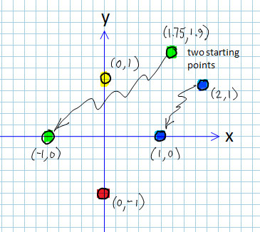
Making a color-coded summary of which starting points go to which solutions.

One way to visualize the overall behavior of an iterative process in two variables is to construct what is known as a “basins of attraction” plot. We start by assigning colors to each of the four solutions, as shown in this figure. Then we run Newton’s method from a large number of different starting points, and keep track of which starting points go to which solutions. The starting point location on the plot is colored according to the solution to which it converged. The final result is a color-coded summary of convergence.

The cover story on the Feb 1987 issue of Science News. (Click to enlarge.)

The result of this process is the image shown on the cover of Science News from 1987. (This was probably my first “15 minutes of fame,” back when fractals were brand new.) Notice that there are large red, green, yellow, and blue regions that are regions of starting points that all go to the same solution. On the diagonal, however, the colored regions are tightly intermingled, indicating that very tiny changes in starting point can lead to drastic changes in the outcome of Newton’s method. This “sensitive dependence to initial conditions” is a hallmark of chaotic behavior, and it captured graphically in the basins of attraction images.

You might be wondering about the different shades of each color. I selected the coloring scheme to reflect the number of iterations it took to get to a solution (to within some pre-defined tolerance). The colors cycle through six shades of each hue, from dark to light and over again, with increasing iteration count. Thus, the dark circles around each of the four solutions contain starting points that all converge to the solution in one iteration of Newton’s method. The slightly less dark region around each of them converge in two iterations, and so forth.

The “boundary” of each color is an extremely complex, fractal shape. In fact, it can be demonstrated that all four colors meet at every point on the boundary!

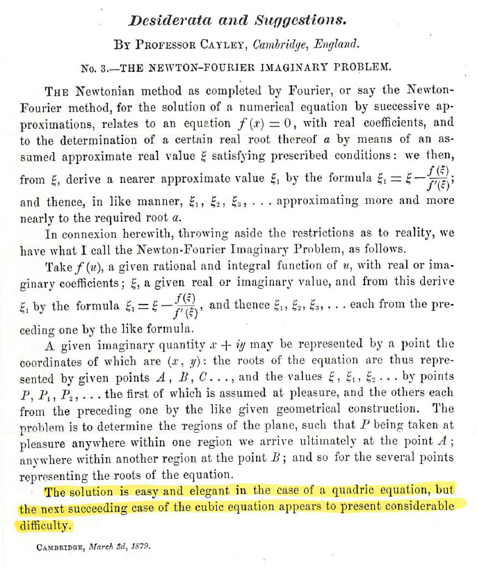
Prof. Arthur Cayley’s paper on the difficulty of describing the behavior of Newton’s method in some cases.

Although fractal images are a relatively recent concept, mathematicians have had glimpses of this behavior for a long time. In the 1800s, Professor Arthur Cayley of Cambridge was studying the behavior of Newton’s method with some very simple equations and found that it was quite difficult to state general rules for associating which starting points end up at which solutions. He wrote a one page paper on the subject in 1879 (shown in the figure). He compared the stable, easy to describe behavior of Newton’s method applied to a quadric (second order equation) to the case of a cubic equation, and observed the latter “appears to present considerable difficulty.” The Science News image above is the case of a fourth-order equation, one degree above the cubic that he considered. The difficulty he was talking about is the behavior in the regions of tightly intermingled colors, where the shapes of those regions defy description.

You might be wondering about the phrase “Newton-Fourier Imaginary Problem.” First the Fourier part: I’m not sure why Cayley is discussing Fourier in this paper. The Newton-Fourier method is known today as a process different from Newton’s method because it adds some additional computation to each step that can improve convergence. But the method he demonstrates in his paper is clearly the basic Newton’s method as I’ve described above.

Regarding the “imaginary” part, he was actually looking at Newton’s method operating on functions of a complex variable, that is, one that contains a real component and an imaginary component containing the imaginary quantity The letter is usually used to denote a complex variable, i.e., Consider the function It has four solutions, just like the example I showed earlier. They are and Newton’s method can be applied just as effectively to functions of a complex variable, and the iteration in this case would be

Interestingly, if a basins of attraction plot were to be made of Newton’s method applied to on the complex plane (real and imaginary axes) instead of the plane, it would be identical to the image on the Science News cover!

Why identical images?

Start with the expression Next, substitute for and expand the fourth power to give (Remember to substitute for every instance of Finally, collect all terms that are real into one equation and all terms that are imaginary into another equation. Divide the out of the second equation, and you’ll be left with the exact same system of equations that I presented earlier; they are equivalent to one another. In fact, the image on the Science News cover is the one on the complex plane, not on the plane!

The Monomial Method

The monomial method is an equation solving technique that I developed back in the ’80s as part of my research activities at the Univ of IL. It grew out of my work in optimization theory, specifically a method known as geometric programming that uses monomial approximations extensively. I found that the monomial method was just as easy to apply as Newton’s method, but was able to solve certain problems in my field of study (civil engineering structures) far more quickly and stably than Newton’s method. I’ll be demonstrating this in an example later.

There are some limitations of the types of problems the monomial method will solve. First, all variables must be positive. There is a logarithmic transformation in the method that will fail if an operating point is not greater than zero. Second, the equations being solved must be algebraic in form, such as All algebraic systems of equations can be cast in the general form

In each of the equations, there are terms, each of which has a coefficient, followed by a product of variables, each raised to a power, The coefficients and exponents can be any real number (positive, negative, fractional, etc.).

Let’s define to be the th term of the th equation, or

Next, we group together all the terms with positive coefficients and those with negative coefficients and recast the system of equations as the difference of two sums of terms, and respectively:

Note that the coefficients in are positive due to the negative sign in the expression. One final manipulation is to bring to the right side of the equation and divide it through, giving us the recast form of the system of equations

I’m hoping to keep this presentation accessible to a wide audience, and I’m sure the math-speak above might be difficult to decipher. So I’ll translate it in the setting of an example with just one equation and one variable:

Using the terminology above, and The recast form is

So in other words, all those math symbols above simply mean “divide the positive terms by the negative terms and set it equal to 1.”

We now apply a process called condensation to and separately. Condensation is the process of approximating a multi-term expression with a single-term expression (also called a monomial). It does this using a famous relationship between the arithmetic mean and the geometric mean of a set of positive numbers

The are weights, or fractional numbers that sum to 1. When all the weights are equal, then the left side is the familiar arithmetic mean (average) of the numbers, and the right side is the less known geometric mean. For example, if and all the geometric mean is and the geometric mean is

The inequality becomes more useful to us if we make the substitution giving

This is where the magic happens. Instead of thinking of the as simple numbers, we can think of them as monomials, just as we’ve defined earlier:

OK, lots of math. But let’s step back here and see what we have. The left side of this expression is simply our familiar expression for or the positive or negative terms in an equation. The right side, after everything gets multiplied out, is simply a single term, a monomial, something like This is a monomial approximation to the polynomial expression on the left. The monomial will exactly equal the polynomial when evaluated at the operating point, and will approximate its value at other values of

So now let’s complete the monomial method, first in words, and later with math. We start by condensing and each to monomials. The ratio of two monomials is again another monomial, so is an expression setting a monomial equal to 1. Remember from high school math that the logarithm of a product of numbers is equal to the sum of the logarithms of the numbers (the basis of the slide rule, for those of you as old as I am). The log of this monomial equation becomes a linear equation, which is simple to solve, giving rise to the new operating point (after transforming back out of log space with the exponential function, ).

The one missing piece to the puzzle is how to handle the weights, It’s pretty simple: they are calculated as the fraction that each term in or contributes to the total, when evaluated at the current operating point. See how this makes the sum of the equal to 1?

It’s time to continue our simple example above. We had and Let’s select an operating point of which gives us these weights:

The +/- superscript on indicates if the term came from or The monomial approximation to is

Taking the log of this gives Solving for gives which leads to This is the new operating point, which completes one iteration of the monomial method. Additional iterations will yield the sequence and a solution has been found.

A Computationally Efficient Way

It is apparent from that last example that the monomial method seems to involve much more computation than Newton’s method. The Newton iteration is simply which generates the series of operating points from :

Although Newton’s method is converging more slowly, the number of computations necessary is far less, especially considering that raising a number to a fractional power takes much more internal computation on a computer than simple multiplication or division.

Fortunately, there is an alternate way to compute the monomial method iteration that is more on par with the computational effort required for Newton’s method. Without getting into the details of the derivation, which are available elsewhere, the monomial method iteration can be stated as the following matrix equation:

where is the change in the log of and the matrix has as its th column and th row the value

For the single variable example earlier, which when evaluated at the operating point gives Since and the right side of the equation is Solving for gives and therefore This version requires far less computation than the monstrous equation used earlier!

Let me restate the math expressions above in words. Recall that each term in and has an associated weight, To create the matrix, simply multiply each exponent, of each variable by the weight associated with the term in which it appears. Gather together these products by common variable and add or subtract the product according to whether the term is in or respectively.

Here’s a two-variable example to demonstrate:

Let’s identify the weights (shown in correspondence to their associated term) as

The matrix will be computed as (rows are by equation and columns are by variable)

If we start with the weights will evaluate as

and matrix will evaluate as

After evaluating the right-hand side [], we have the linear system

which solves for and The new operating point becomes and

Relationship Between Newton’s Method and the Monomial Method

Again, without delving into details that are available elsewhere, the monomial method applied to can be shown to be equivalent to Newton’s method applied to

Note that Newton’s method is operated in the space of instead of in the space of

Newton’s method in matrix form is where is the Jacobian matrix of first partial derivatives. The monomial method can be expressed similarly in terms of partial derivatives as

and in this expression are the Jacobian matrices of the and functions, evaluated at the operating point. The matrices are diagonal matrices (all zeros except the values on the main diagonal): has the values of the operating point, on the diagonal; and have the values of and on the diagonal (and they are inverted, so the diagonals are just and ).

Why Bother?

So it seems the monomial method requires a little more computation. What do we stand to gain?

The following example is what convinced me that I was on to something with the monomial method. It demonstrates that for some applications, the difference in behavior between the monomial method and Newton’s method can be striking. It is most clearly demonstrated by constructing basins of attraction plots, as we did earlier.

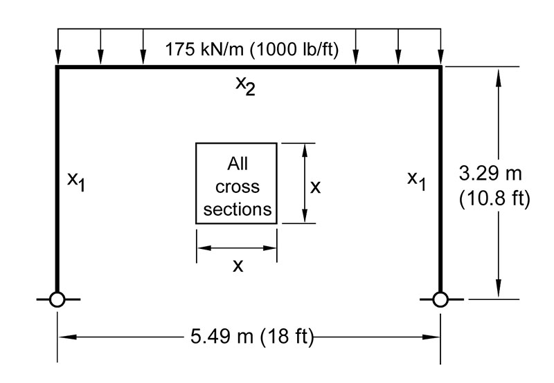
The design of a civil engineering frame structure comprising three members. (Click to enlarge.)

This example comes from the field of civil engineering structural design. One of the simplest frame structures, called a portal frame, has only three members, two vertical columns and a horizontal beam. The design goal is to select the dimensions of the members (the size of their square cross sections) so that the frame safely supports a load of 1000 pounds per foot along the beam. Assuming the two columns are of the same size, there are only two design variables, and that we seek to determine. Without getting into the engineering details, the example presented earlier

are the governing equations for this example. In other words, values of and that satisfy these equations are dimensions of the structure that we seek. These solutions are known as “fully-stressed designs” and can be thought of as particularly good designs because are safe and yet economical because they don’t unnecessarily waste building materials.

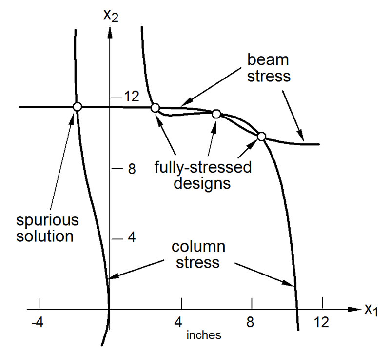
A plot of the two equations being solved. (Click to enlarge.)

We can plot the two equations on the plane, as shown in the figure. The curve that runs more or less horizontally comes from one equation, whereas the two curves running vertically are two “branches” of the other equation. Since the equations are nonlinear, there are several solutions that satisfy them, shown as small circles where the curves intersect. Three of the four solutions fall in the positive quadrant of the “design space,” and represent physically realizable solutions. The fourth solution has a negative value for Although that point formally satisfies the equations, it is not a real solution because the square cross section cannot have a negative dimension. We call that a “spurious” solution.

The three positive solutions have an interesting interpretation from an engineering point of view. The leftmost of the positive designs (with coordinates of approximately and ) has a heavy horizontal beam and relatively slender columns. This design resembles the ancient “post and lintel” type construction, where the beam does most of the work and the columns just prop up the ends of the beam without exerting too much effort. In contrast, the rightmost design has beam and column dimensions that are more similar. In this case, there are substantial forces being developed in the corners of the frame, and much of the load is carried by the bending action transmitted between the beam and the columns. It is a very different sort of load-carrying mechanism, one that is more recent in structural engineering practice with the advent of structurally rigid frame connections. I recall my PhD advisor, Narbey Khachaturian, telling me that the various solutions represent distinct load paths, or preferred ways that the frame likes to “flex its muscles.”

To create basins of attraction plots, we need to assign colors to the four solutions. Going from left to right, let’s select yellow, red, green, and blue. Let’s solve the equations using Newton’s method first. Here are the basins of attraction:

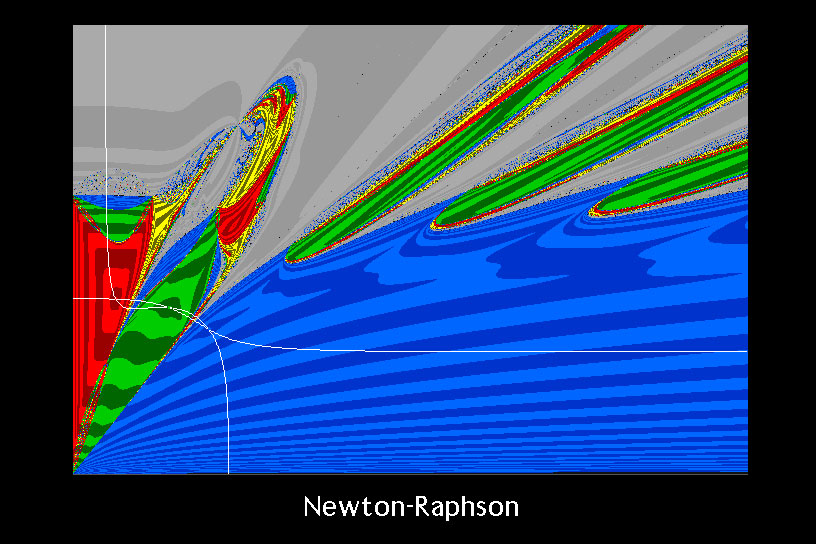
Basins of attraction for the frame example, as solved by Newton’s method. (I created this image decades ago, back when I was still calling it “Newton-Raphson.”)

I’m showing just the positive quadrant of the design space, and the curves are shown in white. The first thing you might notice is the large region of gray. That is a fourth color I selected to indicate when Newton’s method has failed, in this case, due to numerical overflow. In other words, any starting point in a gray region produced a series of operating points that just kept getting bigger and bigger until the computer could no longer represent the numbers and gave up with an error condition.

The two shades of each color represent whether the number of iterations it took to converge (or fail) was odd or even. Thus, the spacing of these stripes gives an indication of how fast the method converges (narrower stripes means slower).

Another interesting observation is all the yellow in the plot. These are starting points that end up at the spurious, meaningless solution, even though the process was initiated from a perfectly reasonable starting point. This is particularly troublesome. There are lots of places where very good initial designs, in the vicinity of the best designs, end up with useless results by Newton’s method!

Now let’s compare this to the monomial method:

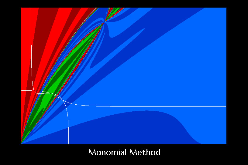
Basins of attraction for the frame example as solved by the monomial method.

What a world of difference! First of all, there are very few starting points that run into numerical difficulty. Second, the spacing between the stripes of color shades are much larger, indicating that convergence is happening very quickly, typically within just a few iterations instead of dozens. Third, and perhaps most importantly, no starting points end up at the meaningless solution (simply because the monomial method can’t converge there).

Special Properties

The monomial method exhibits some unusual properties, not shared by Newton’s method, that are responsible for the improved performance in certain types of applications.

• Multiplication of an equation by a positive polynomial has no effect on the monomial method iteration. With Newton’s method, it is often suggested that equations be put in some sort of “standard form” by multiplying through by powers of the variables. This can improve the performance of Newton’s method in some cases. There is no reason to manipulate the equations in this way for the monomial method. It will give the same sequence of operating points in all cases of this type of manipulation.
• There is an automatic scaling of variables and equilibrating of equations built into the monomial method. Newton’s method benefits greatly from these actions, but they must be done outside of, and in addition to, the regular Newton iteration. By examining the form of the monomial method involving Jacobian matrices (presented earlier), it can be seen that scaling and equilibrating are taking place automatically via the diagonal matrices that pre- and post-multiply the Jacobian matrices.
• The monomial method was shown to be equivalent to Newton’s method applied to expressions of the form When one term dominates the others, then the summation over effectively disappears and only the one term remains. The log and the exp functions cancel each other out, leaving just a linear expression, Since Newton’s method applied to a linear expression gives a solution in just one iteration, the monomial method inherits this behavior.
• When initiating the solution process from a very distant starting point, one term of each equation tends to dominate (assuming the terms in an equation have different powers of ) This makes the system appear to the monomial method as a nearly linear system, and initial iterations move very rapidly toward a solution, in contrast to Newton’s method, which can take dozens of iterations to recover from a distant operating point. This “asymptotic behavior” is evident in the frame example presented earlier. See this paper for details.

Connection to Artwork

The basins of attraction study I conducted at the University of Illinois in the late ’80s sparked my interest in creating abstract art using these methods, leading to my Design by Algorithm business. In particular, one of the early pieces I offered (image #34) was based on the frame example:

This is the frame example solved by another method called “steepest descent.” Can you see the three positive frame solutions? This image also appeared on the cover of a math textbook in the ’90s.

Although I’ve retired this image from the set of currently offered pieces, I have since cropped and rotated this image to form what is now known as Image 78:

The basins of attraction construction has been a fascinating “paintbrush” to work with over the past several decades. I have grown to where I can deliberately design math expressions for desired outcomes and express my artistic intent more fully.

________________________________________

Monomial Method by Scott Allen Burns is licensed under a Creative Commons Attribution-ShareAlike 4.0 International License.