![]()
Published December 25, 2014 by Scott Allen Burns, last updated March 15, 2016

Overview: Vision in Curved Space
I investigate how the visual cues that help us to make sense of the world around us would be noticeably different if we lived in a relatively small spherical universe (a type of 3D curved space that closes on itself). Depth perception would be dramatically different. An object’s apparent size and the parallax caused by binocular vision would no longer have the same relationship to actual distance, and in some cases would be the opposite of what we normally experience. At certain distances, we would experience an unusual perspective distortion that would allow us to see around the sides of objects. If we could see all the way around the curved space, the image of ourselves (seen from the back) could conceivably look much like the cosmic microwave background radiation (CMBR) images that we’ve seen in the news in recent years.
Curved Space
Many of us have been exposed to the notion of curved space, either through discussions in math or science classes concerning non-Euclidean geometry or the theory of relativity, or perhaps we’ve been exposed to it through popular literature, such as the 1965 novel Sphereland, a sequel to the 1884 novel Flatland. Curved space appears flat to inhabitants of the space because light follows the curvature of the space. For a long time now, I’ve wondered how curved space would affect optics and vision of creatures embedded in the space. I recently did some simulations and found some pretty interesting things! This presentation is intended for a general audience; I’ve enclosed more technical discussions in collapsible note containers for those who are interested.
The notion of a curved three-dimensional space is difficult to imagine within our limited three-dimensional world view. To get a handle on it, it is sometimes useful to consider a lower-dimensional version of curved space and generalize what we observe to higher dimensions. Consider a two-dimensional world, where two-dimensional beings (having no thickness) are restricted to live on a spherical surface, as depicted in the banner graphic above. I’ve used MRI images to represent the creatures since their “insides” are not visible to fellow creatures; they can see only the outer perimeters of each other.
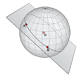
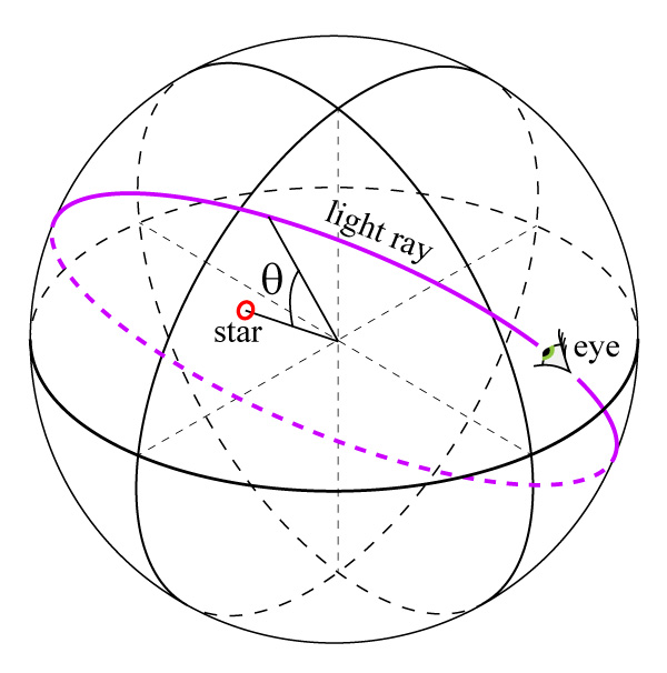
A great circle through points A and B is formed by intersection of the sphere and a plane containing A, B, and the center of the sphere (O).
Let’s discuss a little geometry in the 2D spherical space. A light ray is assumed to travel the shortest distance between two points, which on a spherical surface becomes the portion of the great circle connecting the two points. As usual, the concept of “straight lines” is one that coincides with the paths of light rays. Thus, every great circle is a straight line in spherical space. There are infinitely many straight lines that can emanate from a point, similar to how the lines of longitude emanate from the north or south pole on Earth. Two distinct points determine a unique straight line, unless those two points are exactly on opposite sides of the sphere, in which case there is an infinity of straight lines that connect them. A unique great circle can be constructed through two points on the sphere by constructing a flat plane passing through the two points and also passing through the center of the sphere. If these three points are not collinear (in our external observer’s 3D sense), then there is a unique flat plane that contains them, and the intersection of this plane and the sphere is a great circle.
While it’s fairly easy to picture 2D creatures living in a 2D spherical world, it’s virtually impossible for us 3D-types to imagine how our own space could be curved through a higher dimension, and that if we were to travel far enough in one direction, we would return to where we started. Nevertheless, we can rely on math to predict how this space should appear to us. We can generalize the notion of a great circle and assume that light follows these paths, and from there, predict how these curved light rays would affect our perception of the world.
In reality, we may actually live in a curved space, but one that is so large that we can’t distinguish it from flat space. One way to sense that we live in curved space is to add the three angles in the corners of a triangle. In flat space, they sum to 180 degrees, but in spherical space, they would sum to a larger value. Experiments in outer space show that our space is flat within some small margin of uncertainty, but that doesn’t guarantee that we don’t live in an enormous curved space with a tiny, but not zero, curvature. In this presentation, however, I’m letting the size of the spherical space be relatively small, say, having a diameter of just thousands of times the size of its occupants. I’m also assuming that we can easily see all the way around the universe. That way, visual effects are pronounced and are easy to observe in computational simulations.
I want to clarify that I’m not talking about the curved space of Einstein’s space-time, where massive objects warp the space and produce the phenomenon we call gravity. Instead, I’m considering a fourth spatial dimension, just like the first three, and a 3D spherical subspace embedded in that 4D space. I’m idealizing the curved space to be smooth with constant curvature, so that my computational simulations are easy to perform.
Vision and Perception
The eye’s lens projects a 2D, inverted image of the 3D world around us onto the retina. (Click to enlarge.)
We see the world through lenses in our eyes, which project an inverted image onto our retinas. Although the 3D world around us is presented to our brain in 2D form, the brain’s power of perception interprets various aspects of the projected image to give us the sensation of a 3D environment. These visual “cues” include the size, color, contrast, texture, focus, and relative motion of regions in the 2D projection. We combine these cues with other sensory input (and our experience of the world) to construct a mental image of a 3D world around us. We also gain a sense of relative depth of objects by the way they overlap one another. We take it for granted that as objects gets closer to us, they appear larger.
Speaking of depth perception, another powerful tool for judging depth is our binocular vision. Having two eyes in different locations on our head allows us to view a scene in two slightly different directions. The very subtle differences between these two views is processed by the brain to give a powerful sense of depth, as many of us have experienced in 3D movies.

Both a lens and a pinhole can produce an image. (http://en.wikipedia.org/wiki/en:File:Lens3.svg)
It’s not too difficult to computationally simulate how a lens produces an image through refraction of light rays. Light rays emanating from a point on the object strike the lens and are bent so that they all converge again to a point on the projection plane. But for my purposes, this is all unnecessarily complex. A simple pinhole will also produce an image without the need for considering such things as lens focal lengths and refraction of light. Points on the projection are found by simply tracing the paths of light rays emitted from the object, passing through the pinhole, and falling onto the projection plane. This greatly simplifies the math of constructing a projected image.
Both the lens’s image and the pinhole’s image are upside-down. This is another annoyance that I want to avoid, so I’ll be making use of a different type of projection that has been known for centuries, sometimes called a perspective projection. The idea is that instead of casting a real image onto a projection plane placed behind the pinhole, the projection plane is placed between the object and the pinhole. Then by marking (or calculating) where each light ray intersects the projection plane on its way to the pinhole, an image is constructed on the projection plane. It’s not a real image, like that created by a lens or a pinhole, but a constructed/computed one that closely approximates how the scene appears to the eye, and it’s not inverted. This is demonstrated in the ancient figure shown below.
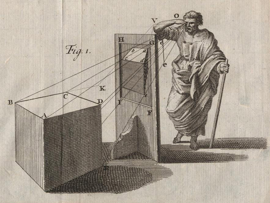
An illustration of how to construct a perspective projection by finding intersections of light rays on a projection plane. From New Principles of Linear Perspective, by Brook Taylor, 1719. By the way, this is the same Taylor as in “Taylor Series Expansion,” for all us engineers who know it well!
A 2D version of the perspective projection on the sphere. (Click to enlarge.)
Perspective Projection: 2D Case
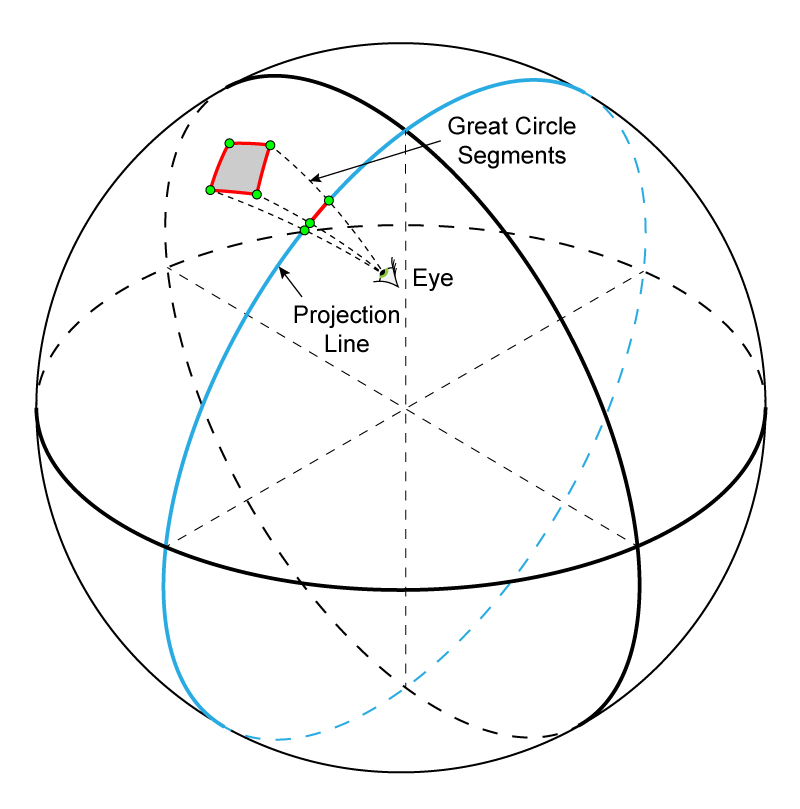
To produce a lower-dimensional analogue of a perspective projection on the sphere, we would pick a particular great circle as a “projection line” (instead of a projection plane, as depicted by the blue circle in the figure) and find where light rays intersect it on their way to the eye.
Each corner of the gray rectangle in this figure has a unique great circle that connects it with the eye. The places where these great circles intersect the projection line form the one-dimensional perspective projection.
This is how the flat creatures would see the rectangle on their one-dimensional retinas. Assuming the gray rectangle is opaque, only three of the four corners will be visible in the projection.
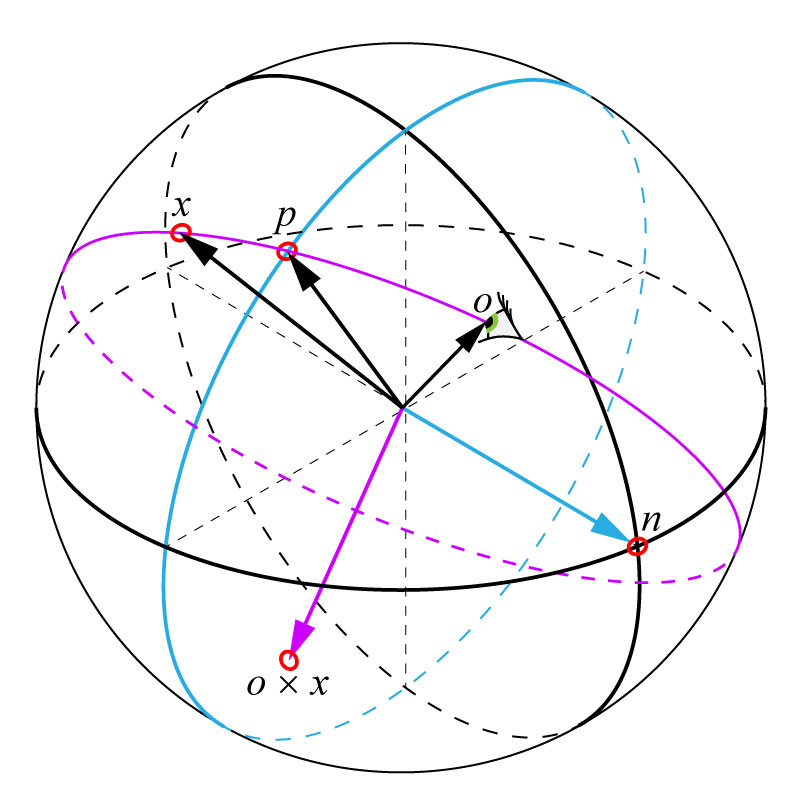
Projection points on the sphere are found with two cross products. (Click to enlarge.)
A little math: The points on the projection line are easily found. Suppose the eye is located at point o and x is a point on the object (e.g., a corner of the rectangle). The point p is the projection point being sought. Assuming the sphere has unit radius, all of these points can also be thought of as unit vectors from the origin. Let q be the normal to the projection line (normal to the plane containing the blue circle), which is defined in advance. The cross product of o and x gives a vector normal to the plane containing the great circle that passes through o and x. Since p lies on both great circles, vector p must be normal to both q and (o × x). It is computed simply as the cross product of (o × x) and q, or p = ((o × x) × q).
Extension to the 3D case
Things get a bit more complicated when considering a 2D perspective projection in the 3D curved space. That blue circle labeled “projection line” shown earlier now becomes a two-dimensional projection plane that is spherical, not circular, and which wraps around the space, and at the same time, stays entirely confined to the 3D spherical surface. It is something that we cannot picture in our minds.
Weird things happen in 4D. For example, in our 3D world, two planes intersect to form a line. But in 4D, two planes intersect in just a single point, analogous to the way that two lines intersect at one point in 2D. It is mind-boggling to think about how this can happen, considering both planes don’t have edges, but extend infinitely! If I begin to feel like I’m getting a handle on visualizing 4D, I just think of this example to remind myself of how woefully inadequate my 3D perception is in this regard! Fortunately, math suffers no such limitations and can manipulate spaces of any dimension with ease.
Projecting points onto a projection plane in curved 3D space is done the same way it was done in the 2D case. Great circles are defined that connect the object and the eye, and the intersections of these great circles and the projection plane are computed.
Math: One complication, however, is that the cross product that was so useful before is not defined for four dimensions. So I had to take a different route. For each point being projected, I defined the plane containing the great circle (connecting the point and the viewer’s eye) by a pair of normals to the plane, giving two equations of the form n1∙x=0 and n2∙x=0. Why two normals? In 4D, an equation of the form n∙x=0 defines a 3D subspace, not a plane. It takes the intersection of two of these 3D subspaces to define a single 2D plane.
The projection plane is defined by q∙x=0, where q is a vector normal to the 3D subspace containing the projection plane. In order to get a 2D projection plane and a 1D great circle, a fourth equation is needed: the requirement that it all takes place on the sphere, i.e., x∙x=1. When this constraint is applied to the 2D plane containing the great circle and the 3D subspace containing the projection plane, it reduces the dimensionality of each. The plane becomes a 1D line (a great circle) and the 3D subspace becomes the 2D projection plane.
The last equation is nonlinear, which results in two solutions. This makes sense because the great circle intersects the projection plane at two points on opposite sides of the sphere. To make the problem linear and simplify the computation, the last equation for the sphere was replaced by an equation for a 3D hypersurface tangent to the sphere, f∙x=1, much the same way that a stereographic projection of a sphere is done in 3D. The point f is chosen to be the center of the projection plane. If we restrict our field of view to the vicinity of the point f, then there won’t be too much distortion in the image. These four linear equations are now sufficient to determine the four coordinates of each projection point p.
I arbitrarily chose the center of the projection plane to be  and the normal to the projection plane to be
  Finding points on the projection plane,
  now becomes a task of solving four linear equations in four unknowns.
![\left[ \begin{array}{cccc} n_1(1) & n_1(2) & n_1(3) & n_1(4) \\ n_2(1) & n_2(2) & n_2(3) & n_2(4) \\ 0 & 0 & 0 & 1 \\ 1 & 0 & 0 & 0 \end{array} \right] \left\{\begin{array}{c}p(1)\\p(2)\\p(3)\\p(4)\end{array}\right\} = \left\{ \begin{array}{c}0\\0\\0\\1\end{array}\right\} &](https://quicklatex.com/cache3/d4/ql_89d8fce5ee05fd220297a1fcc31151d4_l3.png "Rendered by QuickLaTeX.com")
The two vectors  and
and  are two normals to the plane containing (1) the location of eye,
  and (2) the point on the object being projected,
  Since and must be normal to both
  and
and  , they would be expressed as two vectors spanning the null space of the matrix having and as rows.
The null space of a matrix  is the set of all vectors that satisfy
  Try typing “null space {{x1,x2,x3,x4},{o1,o2,o3,o4}}” into Wolfram Alpha. You’ll get a result called “Basis” that shows two vectors that span the null space. These two vectors (or any two that are a linear combination of them) will be suitable for the first two rows of that previous matrix equation for finding the projection point,
I should add a disclaimer. Not being a mathematician, my approach to solving this problem may not be the most direct or elegant. While I’m convinced that my results are correct, it’s very possible that my approach might cause disdain when viewed by a real mathematician, to whom it would be obvious that there is a simpler way of doing this. If that describes you, please contact me with details on how to do it better. I’m always eager to learn new things!
One “constellation” comprising four stars.
To experiment with the projection of objects in curved space onto a projection plane, I first had to define some objects within the space. I sprinkled 50 “constellations” randomly throughout the space, each constellation having four “stars” arranged in a right-handed coordinate system. The stars were colored black, red, green, and blue so that I could visually keep track of the individual stars in a constellation. I defined a four-dimensional coordinate system with the origin at the center of the sphere. Each star has four coordinates, (w,x,y,z), instead of the usual three coordinates of points in our flat 3D space. The four coordinates cannot be arbitrarily chosen, however, because all points must lie on the spherical surface. To enforce this, the sum of the squares of the four coordinates will always equal one (the radius of the space).

A 2D projection of the constellations.
Here is a plot of the random constellations as viewed from outside the sphere. This is how the constellations would appear to a 4D creature if the four dimensions were to be projected on to a two dimensional plane. (I made this figure by simply plotting just two of the four coordinates of each star, which is a simple way of making an orthographic projection.) Although it might appear as though the constellations fill the inside of the sphere, they exist only on the surface. But remember, that “surface” has three independent spatial dimensions.
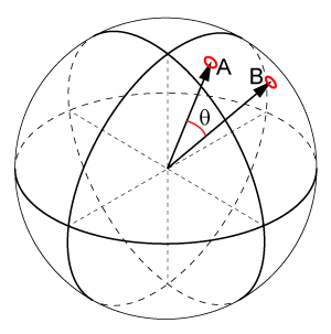
The distance between two points is the angle between them.
I made each constellation the same size. But before we can talk about the size of something, we need to discuss the notion of “distance” in curved space. While it would certainly be possible to define the distance between two points on the sphere to be the arc length along the great circle connecting them, that distance would depend on the radius of the sphere. It is more natural to talk about the angle between the origin-based vectors pointing to the two points. That way, distance is a number between zero and 2π (in radians), where two points on opposite sides of the sphere would be π radians apart.
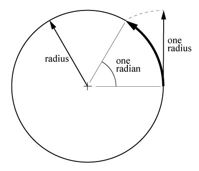 The use of radians is sometimes awkward for those accustomed to measuring angles in degrees. But there is a nice way to think of radians that makes them friendlier. Whenever you see the word “radians,” replace it with the word “radiuses” in your head. A radian sweeps out a distance of one radius that has been curved to lie along the circle. The distance to the opposite side of the circle is a little over three radiuses (3.14, or π of them to be exact), and it takes a little over six radiuses to get all the way around the circle (2π).
Distances greater than pi are meaningful in this context.
It is common for those who study spherical geometry to limit distance between two points to be in the range 0 to π instead of 0 to 2π. They argue that if the angle is more than π, then the angle between the points measured along the other part of the great circle will be less than π, and so the smaller angle should be considered the true distance between the points. In this presentation, however, I am considering light rays that emanate from an object, pass through a projection plane, and enter the eye. Here it is perfectly reasonable to talk about light rays traveling more than halfway around the sphere. It’s true that the object also emanates light in the other direction that reaches the viewer in a shorter distance, but those rays are blocked by the back of the viewer’s head and aren’t seen!
With this idea of distance in mind, the 50 constellations I created are each approximately 0.15 radians across, or about 7% of the diameter of the sphere.
First Glimpses into Curved Space
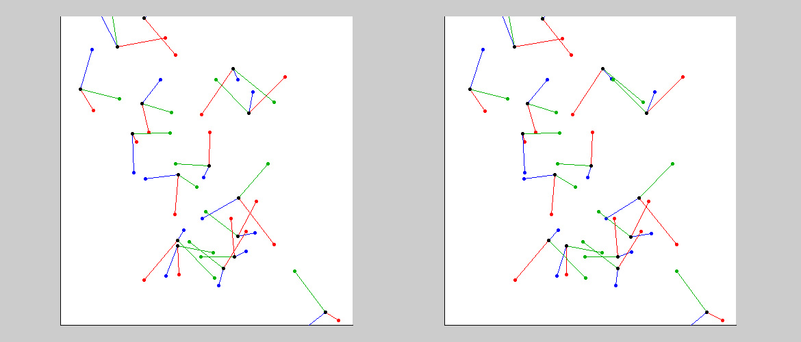
Now that I’ve created constellations to view, the next step is to project them onto a projection plane within the curved space. As discussed previously, this computation involves finding intersections of light rays traveling from the individual stars as they cross the projection plane on their way to the viewer’s eye. The viewer has a limited field of vision, just as a camera with a normal lens can’t see everything around it. The field of view is set up in the calculations to be approximately equal to a normal camera lens (i.e., a 50mm lens on a 35mm camera, equivalent to about a 50 degree field of view). This permits the viewing of about 30% of the constellations.

Perspective projection of a portion of the universe.
Here we see a portion of the universe as it would appear in perspective projection. I constructed this image by finding where each star would project onto the projection plane, and then I added lines to connect adjacent stars. At first, I was concerned that adding these lines might not be legitimate–maybe they would actually appear curved? But upon further reflection, I realized that these lines represent the shortest distance between adjacent stars, which would be great circle segments within the spherical space. Great circle segments must appear as straight line segments to inhabitants of this space, and so their projection would also be straight.
To create this image, I located the viewer’s eye 0.1 radians behind the projection plane. By shifting the eye location slightly to the side and generating a second projection, I can make a stereo pair. In this case, I separated the two viewpoints by 0.03 radians (i.e., the distance between the eyes).
Cross eyes to see the projection in 3D. (Click to enlarge.)
This is a “crossed-eye” version of a stereo pair. To see the illusion of depth, stare at your fingertip placed halfway between your eye and the image. Move your finger forward and back and eventually the two plots will merge into one. (It will actually appear to be three plots, but the central one is the one to focus on.) If you are able to do this, you will clearly see that some constellations are in front or behind others. You can also confirm that the constellations form a right-handed system going red-green-blue.
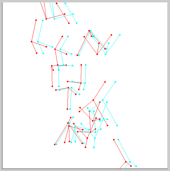
Use red/cyan glasses to get 3D effect. (Click to enlarge.)
It’s difficult for some people to do the cross-eyed stereo view. Another option if red/cyan glasses are available is to look at the plot to the left. If glasses aren’t available, then the animated GIF below should give a sense of the depth.
Roll mouse over to animate. (Numbers are star numbers of central star.)
Recall that I made the constellations all the same size. As expected, they appear in different sizes to the viewer since they are different distances from the projection plane. That’s the normal behavior of a perspective view. What is unusual, however, is that some of the constellations that appear farther away by stereoscopic vision are larger than some of those that appear closer!
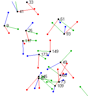
I can add text to the plots that show the distance (in radians) to the central black star of each constellation.

Stereo pair with distances shown (in radians). (Click to enlarge.)
Notice that one of the most distant constellations, at 5.5 radians away, is much larger in appearance than the much closer one at 2.1 radians. Also, the constellations at 1.5 and 4.9 radians away are the smallest in appearance, and yet are on nearly opposite sides of the sphere. The largest constellation appears to be the one at 3.9 radians, more than halfway around the spherical universe from the viewer. What’s going on?
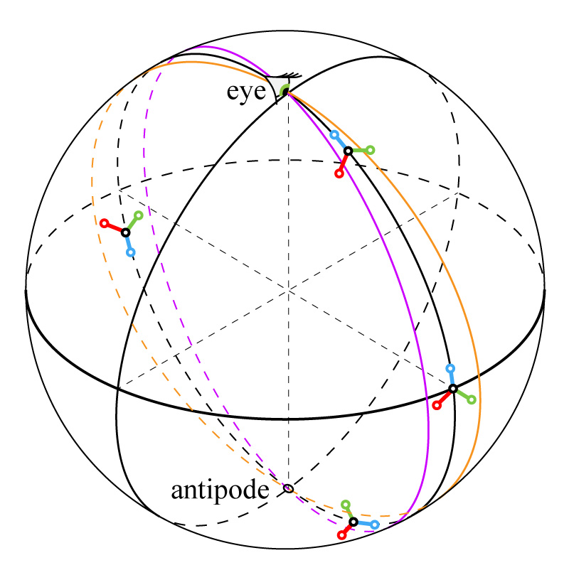
Objects appear smaller as they move away from the viewer, but only within the first quarter of the full tour around the universe. (Click to enlarge.)
It turns out that curved space has an unusual magnifying effect in some regions. Suppose the viewer is located at the north pole, as shown in this figure. Imagine the purple and orange lines to be light rays entering the eye. I’ve drawn several constellations along the direction of view. Compare the size of these constellations to the two light rays. The objects that are near the eye or near the south pole will fill the space between the lines more fully than objects near the equator, and thus, will appear much larger to the viewer.
To check this with the stereoscopic pair shown previously, the equator is a distance of π/2 (1.57) radians from the eye. Indeed, the constellations that are 1.5 and 1.7 radians away are among the smallest. The constellation at 3.9 radians is near the south pole and appears very large. Examining the light rays beyond the south pole on the back side of the sphere, we see that they get farther apart until they reach the equator, and then start to narrow again as they approach the back of the viewer’s head. This means that objects near the equator on the back side, which are near the distance 3π/2 (4.7) radians, should also appear small. Indeed, the plot contains a very small constellation at 4.9 radians. Finally, the constellation at 5.5 radians is very large because it is nearly all the way around the universe, in the region where the two light rays are more closely spaced.
The table below summarizes what has been observed. Note that: “Actual Distance” is measured in the direction of view, so it can be larger than π. “Apparent Size” refers to how large an object is projected onto the viewer’s retina. “Stereoscopic Depth Appearance” refers to the perception of distance as judged by binocular vision.
| Actual Distance in Radians | 0 | π/2 | π | 3π/2 | 2π |
| Apparent Size | large | small | large | small | large |
| Stereoscopic Depth Appearance | near | middle | far | near | middle | far |
The only entry in this table that hasn’t been discussed is the stereoscopic depth appearance in the vicinity of π radians, or near the south pole in the previous figure. Notice in the stereo pair figure how the constellation at 2.4 radians seems so far away and that the one at 3.9 radians seems so close. As an object approaches a point that is on the opposite side of the universe from the viewer, also known as the “antipode,” the image of that object gets larger and larger. As it passes through the antipode from the near side (<π) to the far side (>π), it grows extremely large and stereoscopically distant, then suddenly switches to extremely large and stereoscopically near. It has passed through a singularity. I’ll demonstrate this phenomenon in an animation later, once we’ve developed a way to make more realistic looking views using ray tracing.
In the following section, we’ll be exploring an unusual type of perspective distortion that allows us to see around the sides of objects at certain distances, and we’ll do some more realistic imaging of the constellations using a technique called “ray tracing.”
Perspective Distortion

Very close objects distort in perspective projection.
An unusual aspect of vision in curved space concerns perspective distortion. We’ve all seen photos of people’s faces taken with a fisheye lens that makes their nose large in proportion to other facial features. This type of perspective distortion is avoided in portrait photography by using a longer (mid-telephoto) lens, which makes facial features more natural looking. How does perspective distortion work in curved space?
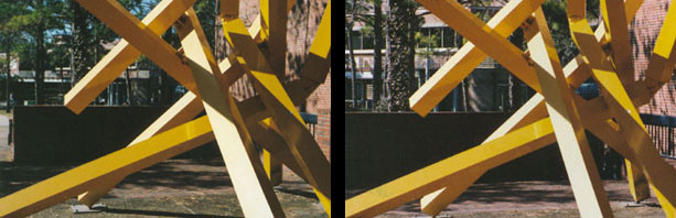
A telephoto lens makes objects at different distances more equal in size.
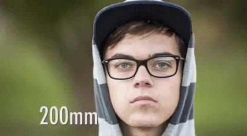
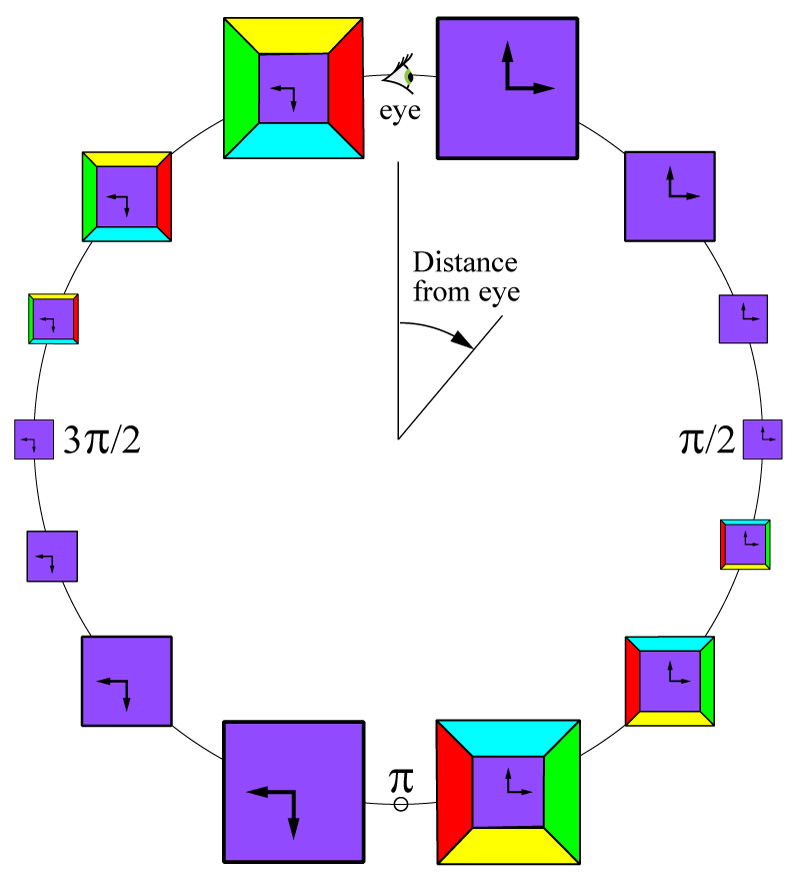
Suppose we are in curved space and have a cube with different colored faces, oriented so that we can see only one face. When the cube is close to us, we can’t see the other five faces; they are all hidden behind the front face. As we move the cube away from us, the lines of sight become more and more parallel. Many of us have experienced this phenomenon in photographs taken with a telephoto lens. Objects in the photo that are at different distances appear more similar in size than in a photo taken with a normal lens. Compare the two photos of the yellow sculpture, taken with a normal lens on the left and a telephoto lens on the right. The building in the background appears much larger with the telephoto lens because the light rays reaching the lens are all more parallel to one another. In the example below, notice how a longer focal length lens lets us see more of the hood material. But with even longer lenses, there would be less and less change, limited by the light rays being parallel in the limiting case for a flat-space universe.
Source: Giphy.com
Returning to the cube example, although we can’t see the back face of the cube, if the cube were translucent, the back face would appear to be getting larger (i.e., more similar in size to the front face) as the cube moves away from us. When the cube reaches a distance of π/2 radians, the light rays reaching us have all emanated from the cube in the same direction, and now we’re seeing the four side faces in edge-view. If we could see the back face, it would appear the same size as the front face. This is the limiting perspective in a flat universe, one we would almost achieve by viewing a very distant object through a powerful telescope. But in a spherical universe, we can go beyond that limiting perspective.
Appearance of a cube as it moves away. (Click to enlarge.)
Moving the cube beyond the 1/4 point (π/2 radians), it begins to grow and we begin to see all four sides in addition to the front face! Think of this as a sort of reverse perspective. Only the back face of the cube is obscured. This is not a phenomenon that we would experience in flat space.
As the cube approaches the halfway point around the universe (our antipode), it gets extremely large, so large that we can’t see all of it in our limited field of view. By the time it has moved far enough past the antipode to be seen in its entirety, we will find that the image has reversed top-to-bottom and left-to-right. It is now seen again in the up-close perspective, where we can see only the front face. Continuing the trip around the universe, the cube shrinks as it approaches the 3/4 point (3π/2 radians), and beyond that, grows again with all four sides being visible, but note from the colors of the sides that it is still reversed in appearance.
Interestingly, if we were to turn around and look at the cube in this most distant position, it would be very large and close, and we would be seeing the back face that has been obscured the whole time that we were facing the other way.

An experimental “UV Mapping” photograph depicting what a face might look like seen across the curved universe. (Photo by Neil Marshall http://www.photoweeklyonline.com/360-degree-portraits/)
Seeing around the sides of an object is a strange concept. I imagine that if we were able to view a person’s face just short of halfway around the universe, it might look something like the experimental “UV mapping” photograph shown here.
Ray Tracing
Modern ray tracing. (By Henrik, via Wikimedia Commons)
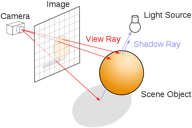
Up to this point, when I’ve prepared an image of objects in curved space, I’ve projected key points, such as the locations of individual stars, onto the projection plane. In recent decades, the computer graphics industry has refined a technique called ray tracing, which can produce extremely realistic images from computer-based solid models. Ray tracing can model lighting effects like shadows, reflections, refractions, translucency, scattering, and dispersion. It is a key element in modern computer animation found in professional feature length films, such as those produced by Pixar.
I’ll be using a relatively simple version of ray tracing. Nevertheless, it requires greatly more computational effort to make an image, growing from mere seconds to make the previous images, to multiple hours for those that are to come. The idea I’ve implemented here is pretty simple. The projection plane is divided into a very fine grid of pixels, and a ray is passed from the viewer’s eye through each pixel. The ray is then observed passing through the space (along a great circle) and a record is kept of which stars it passes near on its path around the universe. The pixel is then colored according to the light ray’s cosmic encounters, and the process is repeated with a new light ray for each new pixel in the projection plane. The end result is a “bitmapped image,” similar to a digital image you’d get from your camera.
The distance between a light ray and a star.
The amount of light that is assumed to return along a light ray path when it encounters a star is based on how closely the ray passes the star. As usual, the distance is measured in terms of the angle that the star makes with the plane containing the light ray’s great circle. That angle,  is shown in the figure to the right. When a light ray passes exactly through a star, the angle is zero, and the maximum amount of light is recorded as returning along the light ray path. When the light ray misses the star, the angle is used in the formula
  where
where  is a sensitivity factor that controls the “spread” of the star’s glow, and overall brightness of the ray-traced image. If the light ray passes multiple stars, the intensities add, which allows the glow of neighboring stars to overlap.
Math: Deriving a formula for the angle between a vector and a plane in 4D proved to be challenging. As usual, I could do it easily in the 3D case but the 4D case was harder to figure out. Eventually, I turned to an online math-help website for assistance. A kind fellow named “Travis” walked me through the math to arrive at the expression below. (discussion) He introduced me to a couple of math concepts I had never heard of before, the “Gramian” and the “wedge product.” Here’s how the formula works: If A and B are two vectors in the plane containing the light ray, and C is the vector pointing to the star, then a matrix comprising the three vectors is constructed and multiplied by its transpose. The determinant of this product is known as the Gramian, and it gives the square of the volume of the parallelepiped with A, B, and C along its sides (which works regardless of the dimensionality of the space in which it resides!).
![{\sin \theta = \sqrt{\dfrac{\det\left( \left[ \begin{array}{ccc} - & A & - \\ - & B & - \\ - & C & - \end{array} \right] \left[ \begin{array}{ccc} | & | & | \\ A & B & C \\ | & | & | \end{array} \right] \right)}{\left[(A \cdot A) (B \cdot B) - {(A \cdot B)}^2\right] (C \cdot C)}}} &](https://quicklatex.com/cache3/91/ql_24d0f6eb0cb11d0f6e551120f877ff91_l3.png "Rendered by QuickLaTeX.com")
The denominator contains an expression for the squared magnitude of the wedge product of A and B, multiplied by the squared length of C. This is essentially a dimension-independent version of how the cross product is used in 3D to compute an angle. This has prompted me to start reading up on wedge products, geometric algebra (not to be confused with algebraic geometry), and something called “Clifford algebra.” These are fascinating concepts, and they came in very handy when I started animating the motion of stars, which I’ll demonstrate later.
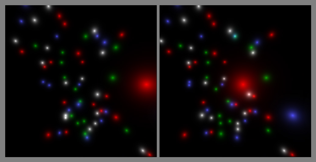
Below, on the left, is the ray-traced version, and on the right a transparent overlay of the previous constellation plot to show the agreement in the two approaches.
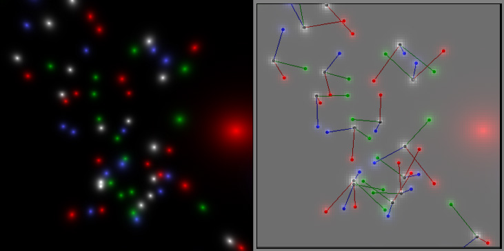
A comparison of the ray traced image and an overlay of the previous imagery.
A very large red star has appeared. The reason for this is that I programmed the earlier plots to ignore constellations that had fewer than two stars appearing in the field of view. This new constellation is an extremely distant one. The red star you see is at a distance of over six radians from the eye, or in other words, it is immediately behind the viewer’s head and is being seen all the way around the universe. Because is it so close to 2π radians away, the constellation is enormous.
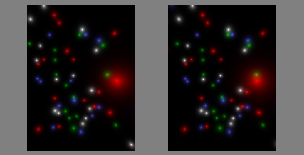
A stereo pair can be produced by shifting the viewpoint slightly.
A stereo pair with an eye separation of 0.03 radians. The effect is difficult to visualize because the large red star is so much more distant. The next figure works better.
The extreme distance of the big red star causes such a large parallax shift that it becomes hard to adjust our eyes to make it seem to “fit” in with the other stars. It’s like trying to view something held up close to our eyes at the same time as viewing a distant mountain. I can reduce the distance between eyes to make the parallax more reasonable for the red star, at the expense of all the other stars appearing somewhat flatter.
By moving the eyes much closer together (0.005 radians), the depth effect is much easier to achieve. (Cross eyes to merge images–click to enlarge.)
The Mollweide Projection
I was getting tired of only seeing a small fraction of the total number of constellations spread out throughout the universe. I started looking into other ways to view a universe, and came across something called the Mollweide projection [pronounced mawl-vahy-duh]. It is most commonly used to view the Earth without too much distortion, as shown below.
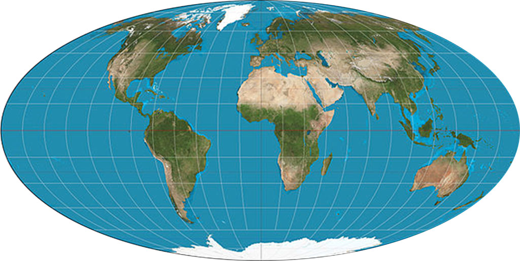
Mollweide projection of Earth. (By Strebe (Own work) [CC-BY-SA-3.0 (http://creativecommons.org/licenses/by-sa/3.0)], via Wikimedia Commons)
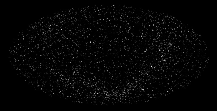
Mollweide projection of sky. (http://astronelson.wordpress.com/2013/01/15/first-light-software-edition/)
Here you can see the Milky Way running through the image like a “smile” and Polaris (the North Star) at the very top. Each point on this map represents a latitude and longitude. The star map associates a longitude and latitude with each star (as though we have frozen the Earth in one place in its rotation about its axis and in its revolution around the Sun). The way to think of this is to imagine that the viewer is situated at the center of the earth. Each point on the surface of the earth (specified by its longitude and latitude) defines a direction of view into the sky.
My goal was to create a Mollweide projection of the 50 constellations I created, so I could see them all at once. But that meant I would have to somehow convert the 4D coordinates, (w,x,y,z), of each star to a latitude (-π/2 to π/2) and longitude (-π to π). After a little Googling, I ran across something called “hyperspherical coordinates.” From Wikipedia:
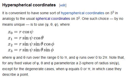
Hyperspherical Coordinates. (http://en.wikipedia.org/wiki/3-sphere)
It seemed like a long shot, but at least it did involve angles that vary over a range of 0 to π and 0 to 2π radians. The quantity φ seemed like the obvious choice for longitude, since it was the only one that had a range of 0 to 2π, but there were two choices for latitude, ψ and θ, both ranging over 0 to π radians. So I took a guess that θ is related to latitude and lucked out! With a little tweaking of signs and ranges, I came up with a simple conversion between 4D coordinates and Earth coordinates.
It took some trial and error to discover that the arbitrary coordinate system I had chosen for the stars and the hyperspherical coordinates defined in Wikipedia were offset in latitude by a phase angle of π/2. But once that was determined, everything else fell nicely into place:
First, a conversion from 4D (represented as vector v) to latitude, longitude, and distance (in Matlab code):
function [latitude, longitude, distance] = lat_lon_dist_from_4D(v)

distance = acos(v(1));

latitude = acos(-v(3)/sin(distance))-pi/2;

longitude = atan2(v(4),v(2));
and then a conversion back to 4D:
function v = lat_lon_dist_to_4D(latitude, longitude, distance)

v(1) = cos(distance);

v(2) = sin(distance)*sin(latitude+pi/2)*cos(longitude);

v(3) = -sin(distance)*cos(latitude+pi/2);

v(4) = sin(distance)*sin(latitude+pi/2)*sin(longitude);
The only remaining task in making a Mollweide plot is the transformation between latitude/longitude and x/y coordinates on the plot. Wikipedia helped here, too (note that the Greek symbols used here are different than those used in hyperspherical coordinates):

Mollweide transformation. (http://en.wikipedia.org/wiki/Mollweide_projection)
The only tricky part is getting the value of θ from φ, which requires an iterative solution. For completeness, I might as well give the reverse transformation from x/y to latitude/longitude:

Mollweide inverse transformation. (http://en.wikipedia.org/wiki/Mollweide_projection)
Armed with these transformations, creating a Mollweide projection of my 50 constellations becomes almost trivial: just take the star coordinates, transform to latitude/longitude, then transform again to x/y, and plot:
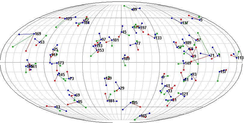
Mollweide projection of the 50 constellations, viewing only from the near side.

Previous view with constellation numbering.
I’ve numbered the constellations according to the star number of the central star. Compare this to an earlier plot with constellation numbers turned on, shown to the right. The field of view from before is located in the left-central portion of the Mollweide plot. But aren’t there are some constellations missing? After a little more examination, you’ll find the missing ones on the right-central portion of the Mollweide plot, turned upside down. At first I thought this was an error in my math, but then it dawned on me that the transformation between 4D coordinates and latitude/longitude always uses the shortest distance to the star. All of the stars that projected into our earlier images with distances greater than π are shown as though the viewer has turned around and is viewing them in the opposite direction, or in other words, has traveled all the way around the Earth to see them from a closer perspective.
With a little more tweaking to the code, I was able to plot stars farther than π radians away as they would be seen all the way around the spherical universe:
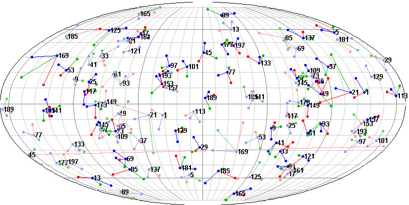
Mollweide projection of the 50 constellation, view each from both the near side and the far side.
The more distant stars are plotted in lighter colors to distinguish them from the closer ones. Now the left-central portion of the Mollweide plot matches the earlier plots.
To help us get our bearings, I can superimpose a map of Earth on this plot.
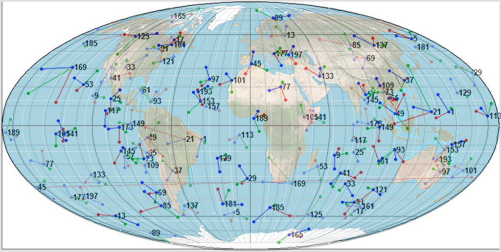
Mollweide projection of the 50 constellations, superimposed over a map of the Earth (to aid in giving directions).
The large constellation labeled 21 that is over South America also appears over the Philippines. Its red star is right above the equator in both views, and it is the large red star we encountered earlier in the first ray-traced images. From South America, we would be seeing the constellation all the way around the spherical universe, whereas from the Philippines, we would be seeing it physically nearer to the Earth (but not any different in apparent size!).
Ray Tracing a Mollweide Projection
In the previous section, I discussed how two of the hyperspherical coordinates, φ and θ, had a very close relationship to latitude and longitude in the Mollweide projection. It turns out that the third coordinate, ψ, is identical to the distance from the viewer (the values I plotted earlier in the stereo pair of constellations). This fact allows me to do ray tracing with ease.

Converting a latitude and longitude on the Mollweide projection to a ray for ray tracing.
For each pixel in the Mollweide projection (which I’ll call the “map” for brevity), a latitude and longitude can be found. Then using two arbitrary distance values, I can compute the 4D coordinates of two points above the point on the map at two different “altitudes.” Two points determine a unique line, or in this case, a unique great circle, which is used as the light ray path for that point on the map. As before, the light ray is tracked around the universe as it encounters stars, and the proximity of the ray to those stars determines the intensity of the map pixel.
In previous ray tracings, I used red, green, blue, and white as star colors to indicate their position in each constellation. I’m going to change the coloring scheme now, since I don’t draw constellation lines in ray-traced imagery. Instead, I’m going to color stars according to their distance from the viewer, ψ.
We’ve all heard cosmologists tell us about how the universe is expanding. Evidence of this comes from measurements showing that the light from distant objects in all directions is shifted toward longer wavelengths, or is “red-shifted.” In the spirit of an expanding universe, I’ve chosen a color scheme that makes near stars bluish, medium range stars white, and distant stars reddish. Here is the result:
The fifty constellations in Mollweide projection, colored blue to red according to distance.
Two constellations stand out. The first is constellation 21, whose big red star we encountered earlier, and constellation 169 over Hawaii and South Africa. Both of these constellations are very near Earth (as seen from Hawaii and the Philippines) and we are also seeing them from the back when we look at them from South Africa and South America. Because of the natural lensing of curved space, all four constellation views are equally spectacular in the sky. On Earth, you’d have to travel around the world to see the opposite side of any given constellation. But floating out in space, all you’d have to do is turn your head around.
In the following section, we’ll add motion to our visualization and animate how it would look for objects to travel all the way around the universe. Finally, we’ll examine how we would see ourselves if we could peer far enough into the sky.
Close Encounters
Emboldened by my success in ray tracing on the Mollweide plot, I decided to try to animate the ray tracing by giving motion to a constellation, i.e., moving it through curved space as a group of four stars. In flat space, this would be a simple computation: I’d simply add a displacement quantity to each star’s coordinates to make them move. But in curved space, the stars have to remain on the spherical surface, so movement is really a rotation about the center of the sphere.
Rotations in 4D are quite bizarre. In 3D, when an object rotates, there is an axis of rotation that stays in place. In 4D, an entire plane stays in place while everything else rotates. We can sort of picture it in 3D if we allow an object to deform, keeping one plane stationary while the rest moves, but there is no such deformation taking place in 4D rotations. It defies our limited 3D perception to picture this type of rotation. Fortunately, math doesn’t share this limitation and can perform 4D rotations we can’t imagine.
Math: My first attempt at rotating stars involved forming a 4×4 rotation matrix, R, transforming one position to another, v’=Rv. I managed to find a nice algorithm for building R, but I had to define the amount of rotation in each of the six rotation planes. When it came to moving a star from one place to another on the sphere, I found it challenging to determine these six rotation amounts. After some additional investigation, I discovered the notion of rotors. Again, I found myself in the world of wedge products and Clifford algebra. A rotor turned out to be an elegant and effective means of rotation. It is sort of like a complex number on steroids, with a scalar part and six “bivector” parts. Here is my code to compute the seven terms of a rotor, which performs a rotation to take vector a into vector b:
function R = ab2rotor(a,b)

% Given two 4D vectors, creates rotor R with seven terms:

% scalar,wx,wy,wz,xy,xz,yz, which rotates vector a into vector b.
% form wedge product

w(1)=a(1)*b(2)-a(2)*b(1);

w(2)=a(1)*b(3)-a(3)*b(1);

w(3)=a(1)*b(4)-a(4)*b(1);

w(4)=a(2)*b(3)-a(3)*b(2);

w(5)=a(2)*b(4)-a(4)*b(2);

w(6)=a(3)*b(4)-a(4)*b(3);
% normalize wedge product

w=w/norm(w,2);
% get angle between a and b from dot product

theta=acos((a'*b)/(norm(a,2)*norm(b,2)));

R(1)=cos(theta/2);

R(2:7)=-w*sin(theta/2);
Now to perform a rotation, a vector is sandwiched between R and R* (which is the same rotor with the sign of the last six terms reversed): b=RaR*. Multiplication of a rotor and a vector is a little tricky, but do-able. Read up on Clifford algebra or geometric algebra to learn more.
Let’s get back to moving a constellation through curved space. I’m going to move constellation 21, the one above the Philippines, away from the earth, so that its fourth star is on a direct collision course with the antipode of our viewing position. All four of the stars in constellation 21 will travel together, but only one of them will pass exactly through the antipode. Once they pass the antipode, they will continue on in the same direction until they return to us, this time approaching from above South America. Here is the animation:
To summarize the action in this animation:
1) The constellation gets smaller as it moves away, until it reaches the 1/4 point around the universe.
2) It then grows in appearance and becomes more whitish in color because both near and far views are becoming more equidistant.
3) The fourth star passes right through the antipode, filling our sky with its light from all directions, as seen from everywhere on Earth.
4) After the fourth star passes the antipode, the remaining three stars make a close encounter with the antipode and do an interesting “dance” in the sky.
5) As the constellation approaches the 3/4 point of the universe, it is again very small in appearance.
6) The fourth star eventually comes very near to earth as the constellation gets very large in the sky, both above South America and also seen all the way around the universe from the Philippines. Note the colors have swapped from what they were initially.
Here’s an interesting lesson from this animation: if we were to live in a spherical universe such as this and a star were to wander through our antipode, and assuming its light isn’t diminished by interstellar dust or other celestial objects, then the star’s light would be focused entirely on earth from all directions and torch us in an instant, similar to how an unlucky ant might find itself at the mercy of a young kid with a magnifying glass on a sunny day.
Let’s Make Galaxies
Our actual universe has stars clustered into galaxies. I thought it would be interesting to do something like this in our curved space, so I generated ten galaxies, each containing 500 stars. The stars in each galaxy were randomly positioned over a small region approximately 0.05 radians (≈3 degrees) across. (I accidentally used a uniformly distributed random number generator instead of a normally distributed one, so the 500 stars in each galaxy ended up being packed into a tiny cube-shaped region. By the time I realized the mistake, I had already done about a week’s worth of computing to get the images, so I decided to just live with it.)
I centered one of the galaxies to contain the position of the viewer’s eye, just as we exist within our home galaxy, the Milky Way. Here is what the ray-traced image of the ten galaxies looks like in Mollweide projection:
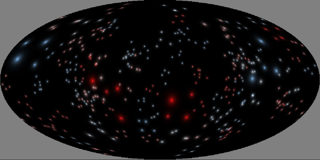
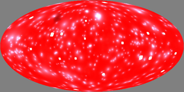
Ten galaxies, each containing 500 stars, ray traced.
The 500 stars of our home galaxy dominate the sky. They are so close and numerous that they block our view of many of the other galaxies. I can adjust the ray tracing algorithm to be less sensitive to light from near sources, allowing us to peer deeper into the universe:
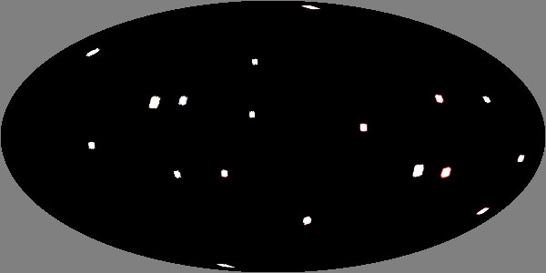
The ten galaxies after adjusting the ray tracing algorithm to be less sensitive to light in proportion to how near the source is.
Now the other nine cube-shaped galaxies are clearly seen, as well as a pervasive red glow seen in all directions from Earth. The red color indicates that this radiation has a very distant source. To determine the cause of this background radiation, I removed our home galaxy from the group of ten galaxies, and recreated the image:
A ray traced image of the remaining nine galaxies, after removing our home galaxy from the dataset.
Interestingly, the deeply red-shifted background radiation is gone, the conclusion being that it is simply an image of home galaxy being seen all the way round the universe! The light we emit passes through our antipode on the opposite side of the universe and continues on until it reaches us again, heavily redshifted due to its lengthy travel. The other nine galaxies, which we see here both in front view in one direction and in rear view from the opposite direction, clearly have very little contribution to the background radiation. I would venture to guess that most of that red background is from the one single star in our home galaxy that happens to be closest to the observer’s viewpoint.
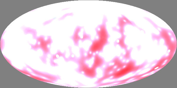
I can further refine the plot of the red glow by ignoring any light that has traveled less than just under 2π radians. This would be analogous to fitting a telescope with a deep red filter that only allows long wavelengths to pass, such a infrared, microwaves, etc. This is plot of just the “backside” of our home galaxy, as seen all the way around the universe. It turns out to have fairly uniform intensity:
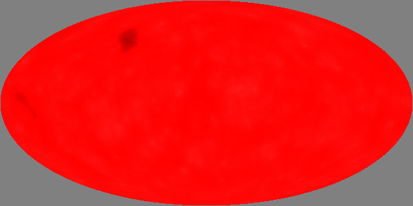
Our home galaxy as seen from all the way around the universe.
I can use a false color mapping to exaggerate the variations in the red cosmic background radiation, where the highest intensities are mapped to reds and yellows, mid-intensities to greens and cyans, and the lowest intensities to blues:
The same dataset shown above, but with a false color mapping applied to intensity.
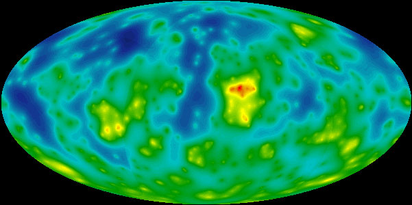
Notice the similarity between this plot and the CMBR (Cosmic Microwave Background Radiation) maps that have been in the news recently:
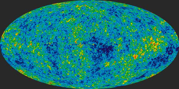
Cosmic Microwave Background Radiation, created by NASA from nine years of satellite data.
The CMBR is thought to be heavily redshifted remnants of the Big Bang. Don’t get me wrong—I’m not suggesting that scientists have it all wrong and that the CMBR is actually just an image of ourselves, as seen all the way around the curved space of our universe. Not being an astrophysicist, I’m sure there are a zillion reasons why that can’t be the case.
To be honest, this is just the result I was hoping for when I embarked on this study. As a youngster, I was fascinated by optics and bought an old overhead projector for $15 from my next door neighbor, Donald Dalle Molle, because it contained a wealth of optical components, including a spherical concave mirror that was used to strengthen the projector’s beam. I was fascinated by staring into the mirror and noticed that if I positioned my eye just right, I could fill my entire field of view with just a reflection of my pupil. I reasoned that this omni-directional reflection should be similar to how light would behave in a spherical universe. So now I can finally bring closure to this idea!
________________________________________

Vision in Curved Space by Scott Allen Burns is licensed under a Creative Commons Attribution-ShareAlike 4.0 International License.
________________________________________