Published March 11, 2021 by Scott Allen Burns; last updated March 12, 2025
3/24/2021 Scope of original paper reduced and surplus material moved here.
3/25/2021 Added plots of high transition solutions for the convexified and truncated CMFs.
3/26/2021 Added comparison of reflectance curves and completed presentation.
4/30/2021 Prefixed figure numbers with “SD-” to distinguish them from the original Article figure numbers.
5/4/2021 Moved most content back to the journal paper upon request of both peer reviewers.
5/10/21 Updated status to show accepted for publication. Fixed figure numbers.
5/24/21 Added notice of publication in CR&A.
3/12/25 Added link to PDF of the Article.
3/12/25 Added discussion of Logvinenko’s “Object Color Solid” publication.
Introduction
This page contains supplementary documentation for the article “The Location of Optimal Object Colors with More Than Two Transitions,” which has been published in Color Research and Application. Any reference to “the Article” on this page refers to this publication. Interested readers may download the Article here: The location of optimal object colors with more than two transitions, Burns 2021
Please note that the content of this supplementary documentation page should not be considered peer reviewed, as it may be updated at any time. This page was last updated on the date shown at the top of the page.
Section 7. Other Illuminants
In Section 7 of the Article, five different highly chromatic illuminants were examined, having chromaticities matching Munsell colors 5R 5/14, 5Y 8/16, 5G 7/10, 5B 6/10, and 5P 4/12. A plot of the chromaticity diagram was presented, showing the high-transition regions associated with each illuminant, plus a sixth equal energy illuminant. Figure SD-1 below presents the same high-transition data shown in Figure 9 of the Article, but plotted on the object color solid (OCS), as viewed from the outside.
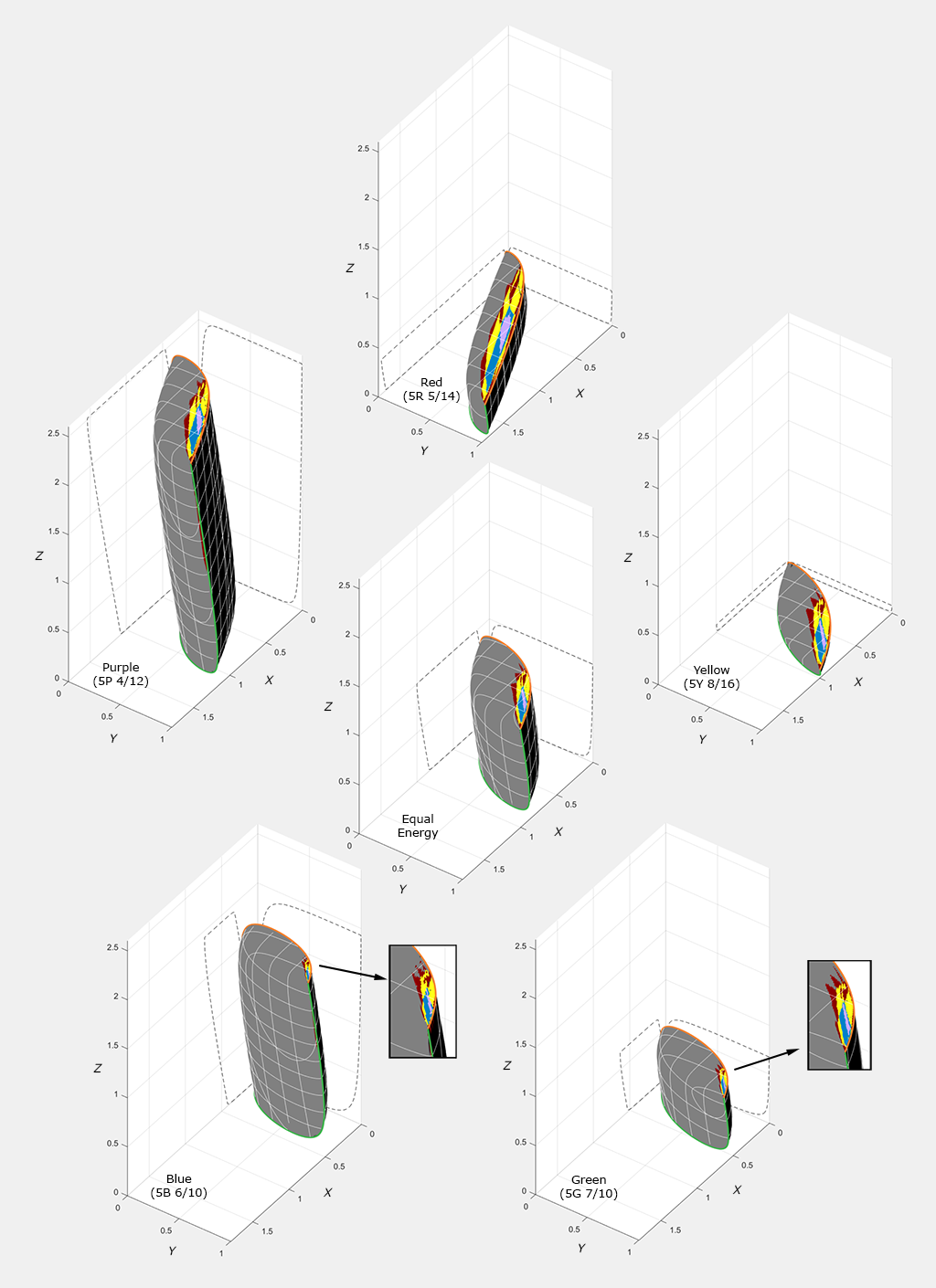
Figure SD-1. The effect of five highly chromatic illuminants on the regions of high-transition optimal colors, as view from the outside of the OCS.
The dashed lines are projections of the OCS onto the XZ and YZ planes. This figure was not included in the Article because the Article was getting too long and figure laden. It is shown here for completeness.
Logvinenko’s “The Object Color Solid” Publication
Subsequent to the publication of the Article, an article was published in 2025 called The Object Color Solid, authored by Logvinenko, Funt, and Bastani. The latter article covers some of the original contributions presented in the prior Article, but does not reference it. For interested readers who wish to obtain the prior Article, they may do so here: The location of optimal object colors with more than two transitions, Burns 2021