Published July 8, 2019 by Scott Allen Burns; last updated Sept 30, 2020

Introduction

This page contains supplementary documentation for the article “Numerical Methods for Smoothest Reflectance Reconstruction,” which has been published in Color Research and Application on November 1, 2019 (online) and December 10, 2019 (print). The paper citation is “Burns SA. Numerical methods for smoothest reflectance reconstruction. Color Res Appl. 2020;45(1):8-21.” The paper PDF appears to be freely available at the journal’s web page, but if not, please contact me if you’d like for me to send you a copy. Any reference to “the Article” on this page refers to this document. The documentation that follows is organized according to the section numbers appearing in the Article.

Please note that the content of this supplementary documentation page should not be considered peer reviewed by the journal, as it may be updated at any time. This page was last updated on the date shown at the top of the page.

---

Section 3. Method 2: Colors Within the Spectral Locus (Real Colors)

Testing Whether a Color is Within the Spectral Locus

Method 2 operates on tristimulus values that fall within the spectral locus. This MATLAB/Octave function will return a logical true/false indicating whether the input XYZ is strictly within the spectral locus:

function in = in_spectral_locus(A, XYZ)
% Checks if XYZ is strictly within the spectral locus.
% Note that the illuminant does not affect the results.
% A is an nx3 array of color matching functions, by columns.
% XYZ is a three-element vector of tristimulus values, any scale; Y > 0.
% in is a logical indicating if XYZ is strictly inside the spectral locus.
locus = A(:,1:2)./sum(A,2); % get x,y of spectral locus
xyz = XYZ/sum(XYZ(:)); % convert XYZ to xyz
[in_or_on, on] = inpolygon(xyz(1), xyz(2), locus(:,1), locus(:,2));
in = in_or_on && ~on;

Some comments:

1. The function computes the projective transformation from XYZ space to the x-y plane, so that the test for being within the locus is reduced a dimension to being within a 2-D polygon.

2. While the shape of the object color solid depends on the illuminant, the location of the spectral locus in the x-y plane is independent of illuminant.

3. Be sure to pass an XYZ triplet that sums to a number far enough from zero to prevent overflow when computing xyz = XYZ/sum(XYZ(:)). The colon allows the input XYZ to be a row or column vector.

4. The resolution of A (number of rows) affects the shape of the computed spectral locus. See Section 6 of the Article for related discussion.

5. The MATLAB/Octave function "inpolygon" returns two logical values: 1) whether a point is either within the polygon or on the boundary of the polygon, called "in_or_on," and 2) whether a point is strictly on the boundary, called "on." Since we are interested in determining if the point is strictly within the polygon, we assess the logical statement "in_or_on && ~on" (in_or_on and not on).

Values of XYZ that return a true value for "in" (logical 1) can be represented by spectral power distributions that are strictly positive. Here are examples of how to use the function:

>> in = in_spectral_locus(A, [0.4, 0.5, 0.6])
in =
  logical
   1

>> in = in_spectral_locus(A, [0.8, 0.2, 0.5])
in =
  logical
   0

________________________________________

Section 3 Correction

It was stated in Section 3 of the Article that "reflectance functions with negative components map to points outside the spectral locus in XYZ space." This is usually true, but not always. Instead, the statement should be been "points outside the spectral locus in XYZ space correspond to reflectance functions with at least one negative component." This is a minor correction and does not affect the development of method 2, which is applicable only to tristimulus values that fall within the spectral locus.

---

Section 4. Method 3: Colors Within the Object Color Solid (Object Colors)

Testing Whether a Color is Within the Object Color Solid

Method 3 operates on tristimulus values that fall within the object color solid. This MATLAB/Octave function will return a logical true/false indicating whether the input XYZ is strictly within the solid:

function in = in_object_color_solid(A, W, XYZ)
% Checks if XYZ is strictly within the object color solid.
% A is an nx3 array of color matching functions, by columns.
% W is an nx1 illuminant vector, any scale.
% XYZ is a three-element vector of tristimulus values, range 0 to 1.
% "in" is a logical indicating if XYZ is inside the object color solid.
n = size(A,1); % resolution of CMFs
Aw = diag(W)*A/(A(:,2)'*W); % illuminant-referenced CMFs
xyz = XYZ/sum(XYZ(:)); % projective transform to x-y space
Y = XYZ(2); % target Y value
% Build a Y slice of object color solid
count = 0;
for step_width = 1:n
    Q = zeros(3,n);
    rho = zeros(n,1);
    % create step function wave rho
    rho(1:step_width,1) = ones(step_width,1);
    for i = 1:n
        % compute TSVs of rho
        Q(:,i) = Aw'*rho;
        % shift rho right with wraparound
        temp = rho(n);
        rho(2:n) = rho(1:n-1);
        rho(1) = temp;
    end
    % look for Q(2) values that straddle Y
    for i = 1:n-1
        % check if Y differences have a change in sign
        if (Q(2,i) - Y) * (Q(2,i+1) - Y) <= 0
            % interpolate to find where line segment crosses Y plane
            Xval=(Q(1,i+1)-Q(1,i))*(Y-Q(2,i))/(Q(2,i+1)-Q(2,i))+Q(1,i);
            Zval=(Q(3,i+1)-Q(3,i))*(Y-Q(2,i))/(Q(2,i+1)-Q(2,i))+Q(3,i);
            count = count + 1;
            x(count) = Xval/(Xval+Y+Zval);
            y(count) = Y/(Xval+Y+Zval);
        end
    end
end
% Q not in order, so find convex hull to sort xy in CCW order
K = convhull(x, y);
x = x(K);
y = y(K);
% check if xyz is within object color slice
[in_or_on, on] = inpolygon(xyz(1), xyz(2), x, y);
in = in_or_on && ~on;

The object color solid boundary is constructed here by a brute-force approach, considering all possible "optimal" colors. First, a 0-1 step function is constructed of varying width (from one wavelength band to all n bands), and then each step function is shifted along the wavelength axis (with wraparound) to produce n shifted versions. This produces n^2 reflectance functions and all optimal colors that can be represented with n wavelength bands. As each step function is shifted, we check if the Y tristimulus values corresponding to adjacent step functions straddle the target Y value. If so, linear interpolation is used to estimate the (x,y) values of the intermediate color at the intersection with the target Y plane. These (x,y) coordinates are collected, and a convex hull function is used to sort the object color solid slice in CCW order. Finally, as with the previous function, inpolygon is used to assess if the input color is within the Y-slice polygon.

Values of XYZ that return a true value for "in" (logical 1) can be represented by reflectance distributions that are strictly between 0 and 1, representing object colors. Here are examples of how to use the function (using an equal energy illuminant that is compatible with a 36x3 A matrix):

>> W = ones(36,1);

>> in = in_object_color_solid(A, W, [0.4, 0.5, 0.6])
in =
  logical
   1

>> in = in_object_color_solid(A, W, [0.2, 0.7, 0.5])
in =
  logical
   0

---

Sections 3 and 4: Python Implementation of Methods 2 and 3

All source code presented in the Article is written in the MATLAB/Octave language. Since publication of the Article, methods 2 (for real colors) and 3 (for object colors) have been implemented in the Python programming language as well. These implementations are available here. This web page also includes Python source code for checking if a color is within the spectral locus, or if it is within the object color solid.

________________________________________

Implementation Note

If programming method 2 or 3 outside the MATLAB/Octave environment, and using an implementation of the LAPACK library for linear algebra (such as the linalg.solve function in the Python SciPy package), be sure to set the "assume_a" input argument to "sym" to indicate that the square matrix is symmetric. This will speed up the computation. Also, the Python SciPy package is dependent on the NumPy package. It is important to install the "Numpy+MKL" version of NumPy, which is linked to the Intel Math Kernel Library and includes required DLLs in the numpy.DLLs directory, and uses an optimized BLAS (Basic Linear Algebra Subprograms) library. The SciPy functions for linear algebra will solve MUCH faster this way.

---

Section 5. Comparison to Measured Object Reflectances

Comparison to Liquitex Paints

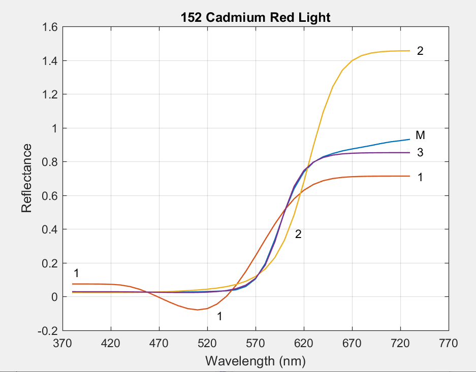
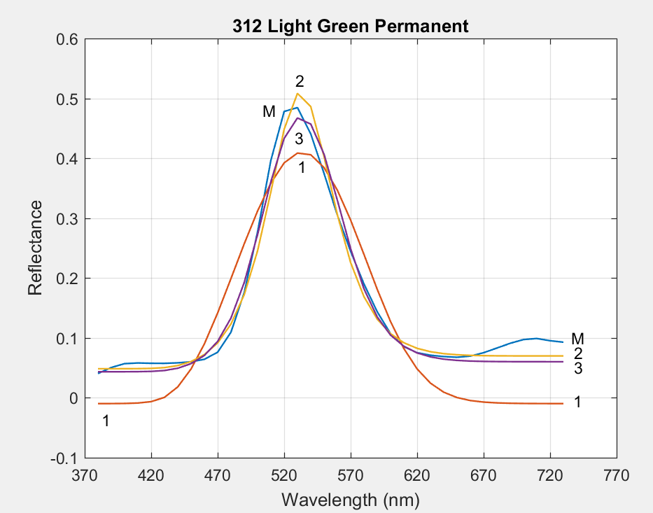
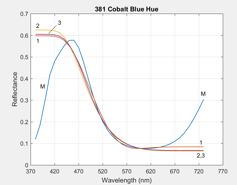
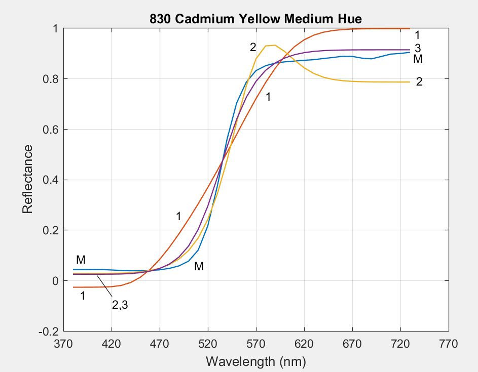
Section 5 of the Article compares the measured reflectance curves of 1485 Munsell Book of Color samples to the reconstructed reflectances of the three methods. Here we compare the three methods to reflectances measured by Zsolt M. Kovacs-Vajna for six highly chromatic Liquitex paints. Since the paint obtained directly from the tube is often highly concentrated and dark, each is mixed with white to achieve maximum chroma before being measured. The following plots show the original measured reflectance curves (blue, lableled 'M'), and the reconstructed reflectances from the three methods (red=1, orange=2, purple=3). Click on an image to enlarge.

________________________________________

Comparison to Li & Luo's implementation of van Trigt's Method

The three methods in the Article are based on work by van Trigt, who developed the objective function to minimize slope squared over the visible wavelengths. In his "unconstrained" formulation, the only constraint imposed on the solution ensures that the triplet of tristimulus values computed from the reflectance reconstruction matches the desired target triplet. In regions of the object color solid where the unconstrained solutions have values outside the 0-1 range, van Trigt introduced equality constraints to enforce that remains in the range 0-1. He also constrained the system so that the slope of the reconstruction is continuous everywhere. Implementing his method requires that 16 different cases be considered.

To simplify this task, Li and Luo solved the problem using numerical optimization, replacing the equality constraints with inequality constraints, . This change mades the problem easier to solve, but introduces the possibility of slope discontinuities in the solution at points where the inequality constraints transition from active to inactive or vice versa. In some cases, slope discontinuities can give the reconstructed reflectance curve an unnatural, truncated appearance. The remainder of this section examines the solutions produced by Li/Luo's implementation of van Trigt's method (called vTLL here) in comparison to the Article's method 3 solutions.

The quantity was introduced in the Article as a measure of how well a reflectance curve matches a reconstructed one with the same tristimulus values, weighted by the luminosity curve () to give more emphasis to the wavelengths to which the eye is more sensitive, and finally normalized by dividing by the number of wavelength bands, :

(1)  

Method 3 and vTLL were applied the to tristimulus values of the 1485 Munsell colors and the resulting values were compared,

(2)  

This is plotted below, after sorting the 1485 results in increasing order:

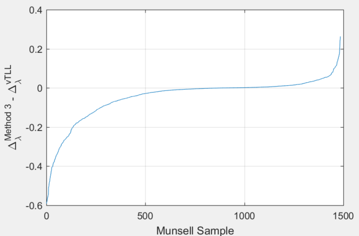
Negative differences are for Method 3 performing better than vTLL and positive differences are for the converse. If we measure the area under both regions of the graph, representing a cumulative amount of difference, we find that the area of the negative region (method 3 performing better) is 5.7 times the area of the positive region (method 3 performing worse), demonstrating that method 3 generates substantially less cumulative reflectance discrepancy compared to the vTLL method when applied to the Munsell colors. Figures 3 and 4 of the Article present examples of the differences in the vTLL solution vs the method 3 solution.

Further discussion of the differences between method 3 and vTLL can be found here.

---

Section 7. Relationship to Matrix R Theory

(This section is being re-written as a full research paper.)

---

References

[1] Trigt CV. Smoothest reflectance functions. I. Definition and main results. J Opt Soc Am A. 1990;7(10):1891-1904.

[2] Trigt CV. Smoothest reflectance functions. II. Complete results. J Opt Soc Am A. 1990;7(12):2208-2222.

[3] Li C, Luo MR. The estimation of spectral reflectances using the smoothness constraint condition. Proceedings of IS&T/SID Ninth Color Imaging Conference, Scottsdale, Arizona, November 1999. 2001:62-67.